Analyse DPE : Carte interactive et statistique

📦 Chargement des packages

library(sf)
library(dplyr)
library(ggplot2)
library(leaflet)
library(classInt)
library(RColorBrewer)
library(car)
library(htmlwidgets)  # Pour saveWidget
library(knitr)
library(kableExtra)
library(ggspatial)

🗺 Cartographie

Pré-traitements

# Chemin vers le fichier
chemin_gpkg <- "G:/UAPV/M1/STAGE/DPE/gpkg/DPE.gpkg"

# Lecture
data <- st_read(chemin_gpkg)

Reading layer `DPE' from data source `G:\UAPV\M1\STAGE\DPE\gpkg\DPE.gpkg' using driver `GPKG'
Simple feature collection with 3240 features and 225 fields
Geometry type: POINT
Dimension:     XY
Bounding box:  xmin: 830791.1 ymin: 6307228 xmax: 868499.4 ymax: 6341774
Projected CRS: RGF93 v1 / Lambert-93

# Création géométrie si nécessaire
if (all(is.na(st_geometry(data)))) {
  data <- st_as_sf(
    data,
    coords = c("coordonnee_cartographique_x_ban", "coordonnee_cartographique_y_ban"),
    crs = 2154  # Lambert 93
  )
}

# Reprojection en WGS84
data <- st_transform(data, crs = 4326)

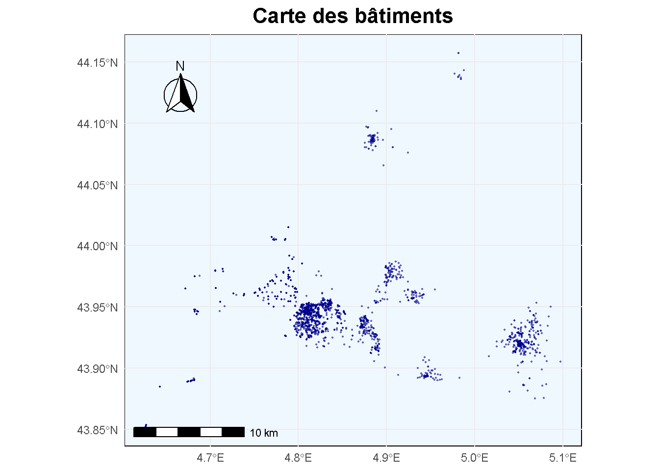
# Plot amélioré avec ggplot2 + ggspatial
ggplot(data) +
  geom_sf(color = "darkblue", fill = "lightblue", alpha = 0.5, size = 0.3) +
  annotation_scale(location = "bl", width_hint = 0.3) +   # échelle en bas gauche
  annotation_north_arrow(location = "tl", which_north = "true",
                         pad_x = unit(0.75, "cm"), pad_y = unit(0.75, "cm"),
                         style = north_arrow_fancy_orienteering) +  # flèche nord top-left
  ggtitle("Carte des bâtiments") +
  theme_minimal() +
  theme(
    plot.title = element_text(hjust = 0.5, size = 16, face = "bold"),
    panel.background = element_rect(fill = "aliceblue")
  )

Paramétrage de la carte

# Chemin vers le fichier
chemin_gpkg <- "G:/UAPV/M1/STAGE/DPE/gpkg/DPE.gpkg"

# Lecture
data <- st_read(chemin_gpkg)

Reading layer `DPE' from data source `G:\UAPV\M1\STAGE\DPE\gpkg\DPE.gpkg' using driver `GPKG'
Simple feature collection with 3240 features and 225 fields
Geometry type: POINT
Dimension:     XY
Bounding box:  xmin: 830791.1 ymin: 6307228 xmax: 868499.4 ymax: 6341774
Projected CRS: RGF93 v1 / Lambert-93

# Vérification géométrie
#print(st_geometry_type(data))

# Création de la géométrie si nécessaire
if (all(is.na(st_geometry(data)))) {
  data <- st_as_sf(
    data,
    coords = c("coordonnee_cartographique_x_ban", "coordonnee_cartographique_y_ban"),
    crs = 2154  # Lambert 93
  )
}

# Reprojection en WGS84 pour Leaflet
data <- st_transform(data, crs = 4326)

# Encoder A-G en numérique
data$etiquette_num <- as.numeric(factor(data$etiquette_dpe, levels = c("A","B","C","D","E","F","G")))

# Jenks natural breaks
jenks <- classIntervals(data$etiquette_num, n = 7, style = "jenks")
print(jenks)

style: unique
  one of 1 possible partitions of this variable into 7 classes
[0.5,1.5) [1.5,2.5) [2.5,3.5) [3.5,4.5) [4.5,5.5) [5.5,6.5) [6.5,7.5] 
       64       187      1064      1167       410       225       123 

# Classe selon Jenks
data$etiquette_class <- cut(
  data$etiquette_num,
  breaks = jenks$brks,
  labels = c("A","B","C","D","E","F","G"),
  include.lowest = TRUE
)

# Palette
palette <- rev(brewer.pal(7, "RdYlGn"))
pal <- colorFactor(palette, levels = c("A","B","C","D","E","F","G"))

# Vérifier
table(data$etiquette_class)

   A    B    C    D    E    F    G 
  64  187 1064 1167  410  225  123 

Création de la carte interractive

# Charger les théâtres
theatres <- st_read("https://raw.githubusercontent.com/Mercatorien/ICU_FESTIVAL_AVIGNON/cf858dbc7d91557000005091c6682346240cc6dc/geodata/theatres.geojson") %>%
  st_transform(crs = 4326)

Reading layer `theatre' from data source 
  `https://raw.githubusercontent.com/Mercatorien/ICU_FESTIVAL_AVIGNON/cf858dbc7d91557000005091c6682346240cc6dc/geodata/theatres.geojson' 
  using driver `GeoJSON'
Simple feature collection with 35 features and 28 fields
Geometry type: POINT
Dimension:     XY
Bounding box:  xmin: 4.628269 ymin: 43.85401 xmax: 5.052309 ymax: 44.13829
Geodetic CRS:  WGS 84

# Carte leaflet mise à jour
m <- leaflet(data) %>%
  addProviderTiles(providers$OpenStreetMap) %>%
  addCircleMarkers(
    radius = 5,
    color = "black",           # Contour noir
    weight = 0.5,              # Épaisseur du contour
    fillColor = ~pal(etiquette_class),  # Couleur de remplissage
    stroke = TRUE,             
    fillOpacity = 0.8,
    popup = ~paste(
      "<b>Étiquette DPE :</b>", etiquette_dpe, "<br>",
      "<b>Année construction :</b>", annee_construction
    )
  ) %>%
  # Ajout des théâtres
  addCircleMarkers(
    data = theatres,
    radius = 6,
    color = "white",    # Contour blanc
    weight = 1.5,       # Contour plus épais
    fillColor = "black",
    fillOpacity = 1,
    stroke = TRUE,
    popup = ~paste("<b>Nom :</b>", nom_t)
  ) %>%
  addLegend(
    "bottomright",
    pal = pal,
    values = ~etiquette_class,
    title = "Étiquette DPE<br>● Théâtres",
    opacity = 1
  )

# Afficher la carte
m

Enregistrer la carte en HTML

saveWidget(m, file = "G:/UAPV/M1/STAGE/DPE/carte_dpe.html")

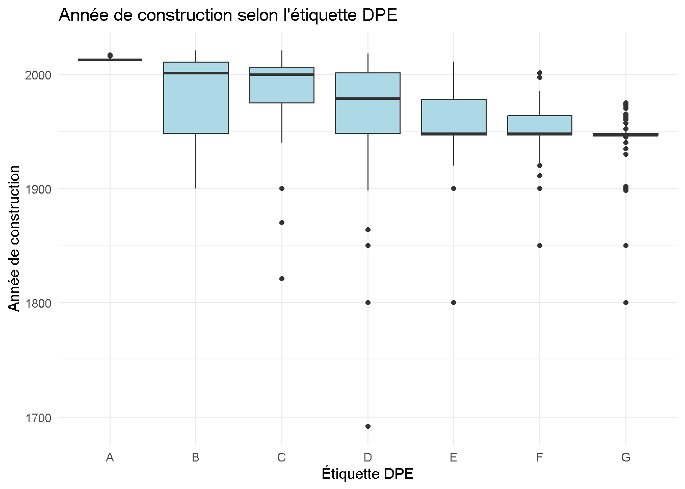
📈 Boxplot des classes DPE par rapport à l’année de cosntruction

ggplot(data, aes(x = etiquette_dpe, y = annee_construction)) +
  geom_boxplot(fill = "lightblue") +
  theme_minimal() +
  labs(
    title = "Année de construction selon l'étiquette DPE",
    x = "Étiquette DPE",
    y = "Année de construction"
  )

Calcul des stats descriptives

stats_summary <- data %>%
  st_set_geometry(NULL) %>%    # retirer la géométrie
  group_by(etiquette_dpe) %>%
  summarise(
    Moyenne = round(mean(annee_construction, na.rm = TRUE), 0),
    Mediane = round(median(annee_construction, na.rm = TRUE), 0),
    `Écart-type` = round(sd(annee_construction, na.rm = TRUE), 1),
    .groups = "drop"
  )

# Affichage du tableau avec kable
kable(stats_summary, 
      caption = "Statistiques descriptives de l'année de construction par classe DPE",
      align = c("c", "c", "c", "c")) %>%
  kable_styling(full_width = FALSE, position = "center")

Statistiques descriptives de l'année de construction par classe DPE

etiquette_dpe	Moyenne	Mediane	Écart-type
A	2013	2013	0.6
B	1987	2001	29.6
C	1989	2000	27.1
D	1974	1979	31.1
E	1958	1948	29.9
F	1946	1948	24.9
G	1943	1947	25.5

ANOVA

Test du lien statistique entre la classe DPE (variable catégorielle), et l’année de construction (quantitative continue)

Tests préalables : Shapiro-Wilk (distribution normale) et Levene (égalité des variances, homocédasticité)

shapiro_results <- by(data$annee_construction, data$etiquette_dpe, shapiro.test)
print(shapiro_results)

data$etiquette_dpe: A

    Shapiro-Wilk normality test

data:  dd[x, ]
W = 0.17214, p-value < 2.2e-16

------------------------------------------------------------ 
data$etiquette_dpe: B

    Shapiro-Wilk normality test

data:  dd[x, ]
W = 0.81064, p-value = 1.277e-13

------------------------------------------------------------ 
data$etiquette_dpe: C

    Shapiro-Wilk normality test

data:  dd[x, ]
W = 0.81982, p-value < 2.2e-16

------------------------------------------------------------ 
data$etiquette_dpe: D

    Shapiro-Wilk normality test

data:  dd[x, ]
W = 0.8553, p-value < 2.2e-16

------------------------------------------------------------ 
data$etiquette_dpe: E

    Shapiro-Wilk normality test

data:  dd[x, ]
W = 0.891, p-value = 1.04e-14

------------------------------------------------------------ 
data$etiquette_dpe: F

    Shapiro-Wilk normality test

data:  dd[x, ]
W = 0.86391, p-value = 1.417e-11

------------------------------------------------------------ 
data$etiquette_dpe: G

    Shapiro-Wilk normality test

data:  dd[x, ]
W = 0.65568, p-value = 2.268e-13

# Test de Levene
levene <- leveneTest(annee_construction ~ etiquette_dpe, data = data)
print(levene)

Levene's Test for Homogeneity of Variance (center = median)
        Df F value    Pr(>F)    
group    6  19.392 < 2.2e-16 ***
      2496                      
---
Signif. codes:  0 '***' 0.001 '**' 0.01 '*' 0.05 '.' 0.1 ' ' 1

ANOVA

# ANOVA
anova_result <- aov(annee_construction ~ etiquette_dpe, data = data)
summary(anova_result)

                Df  Sum Sq Mean Sq F value Pr(>F)    
etiquette_dpe    6  620310  103385   127.1 <2e-16 ***
Residuals     2496 2029583     813                   
---
Signif. codes:  0 '***' 0.001 '**' 0.01 '*' 0.05 '.' 0.1 ' ' 1
737 observations effacées parce que manquantes

Kruskal-Wallis (test non paramétrique)

kruskal <- kruskal.test(annee_construction ~ etiquette_dpe, data = data)
print(kruskal)

    Kruskal-Wallis rank sum test

data:  annee_construction by etiquette_dpe
Kruskal-Wallis chi-squared = 717.95, df = 6, p-value < 2.2e-16

---

Résultat

Interprétation des résultats de l’ANOVA

Note

Contexte :
Nous analysons la relation entre l’année de construction des bâtiments et leur classe DPE (A à G).

Tests préalables

• Normalité (Shapiro-Wilk) :
  Les distributions par classe ne respectent pas la normalité (p-values très faibles, < 0.001).

• Homogénéité des variances (Levene) :
  Les variances sont significativement différentes entre classes (p-value < 0.001).

Résultats principaux

• ANOVA :
  Malgré les violations des hypothèses, l’ANOVA montre une différence très significative entre les moyennes des années de construction des classes DPE (p-value < 0.001).

• Test non paramétrique (Kruskal-Wallis) :
  Confirme cette différence significative, sans supposer la normalité (p-value < 0.001).

Conclusion

L’année de construction est liée à la classe DPE : les bâtiments mieux classés (A, B) sont en moyenne plus récents que ceux classés plus bas (F, G). Ces résultats sont robustes même si les hypothèses classiques de l’ANOVA ne sont pas toutes respectées.